Backpropagation in Neural Networks

Backpropagation of Gradients

Layer ( l) values in the neural network after applying activation function is stored in a column vecotr ( {a}^l). The subscript represent the layer number. The connections are stored in a weight matrix ( W^l ), and the bias column vector is assumed to be ( b^l). The forward propagation is then obtained as

</p>

$$a^l=\sigma (W^l{a}^{l-1}+b^l)$$

We introduce a new vector $z^l=W^l{a}^{l-1}+b^l$, which is the layer $l$ values before applying the transfer function $\sigma ()$. In summary, the neural network procedure is summarized as $$a^l=\sigma (z^l)$$ $$z^l=W^l{a}^{l-1}+b^l$$

To simplify the procedure, we assume a simple 3 layer network as

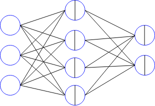
In this network, we have

• Input: $a^0$
• Layer1: $z^1=W^1{a}^0+b^1$ and $a^1=\sigma (z^1)$
• Layer2: $z^2=W^2{a}^1+b^2$ and $a^2=\sigma (z^2)$

where the dimensions are $[W^1{]}_{4\times 3}$, $[W^2{]}_{2\times 4}$, also $[a^0{]}_{3\times 1}$, $[a^1{]}_{4\times 1},[b^1{]}_{4\times 1},[z^1{]}_{4\times 1}$, and $[z^2{]}_{2\times 1},[a^2{]}_{2\times 1}$. Our objective is minimize the distance between the network's output $a^2$ and $t$. A simple cost function here would be $C=\frac{1}{2}||a^2-t|{|}^2$. The weights matrix and bias vectors are updated usinng gradient descent method, where we need to find the derivatives of the loss function with respect to the weights and biases as

$$W^l=W^l-\alpha \frac{\partial C}{\partial W^l},b^l=b^l-\alpha \frac{\partial C}{\partial b^l},l=\{1,2\}$$

We start by finding the derivatives of the weights w.r.t $W^2$, we have $$\frac{\partial C}{\partial W^2}=(a^2-t)\frac{\partial a^2}{\partial W^2}=(a^2-t)\circ {\sigma }^{\prime }(z^2)\frac{\partial z^2}{\partial W^2}=(a^2-t)\circ {\sigma }^{\prime }(z^2)\frac{\partial W^2{a}^1+b^2}{\partial W^2}$$ where $A\circ B$ is the entry-wise product (i.e. $(A\circ B{)}_i=A_i{B}_i$). We further simplify the above relation as $$\frac{\partial C}{\partial W^2}=[(a^2-t)\circ {\sigma }^{\prime }(z^2)][a^1{]}^{\mathrm{\top }}={\delta }^2[a^1{]}^{\mathrm{\top }},{\delta }^2\equiv (a^2-t)\circ {\sigma }^{\prime }(z^2)$$

Notice that the dimensions work out perfectly as

$${\left[\frac{\partial C}{\partial W^2}\right]}_{2\times 4}={\left[{\delta }^2\right]}_{2\times 1}{\left[a^1\right]}_{4\times 1}^{\mathrm{\top }}$$

Furthermore, we need to calculate the derivatives with respect to $b^2$, where we similarly find that

$${\left[\frac{\partial C}{\partial b^2}\right]}_{2\times 1}=(a^2-t)\circ {\sigma }^{\prime }(z^2)\frac{\partial W^2{a}^1+b^2}{\partial b^2}={\left[{\delta }^3\right]}_{2\times 1}$$

Now, we take the derivatives with respect to $W^1$, we find

$$\begin{array}{c}\frac{\partial C}{\partial W^1}=(a^2-t)\frac{\partial a^2}{\partial W^1}=[(a^2-t)\circ {\sigma }^{\prime }(z^2)]\frac{\partial z^2}{\partial W^1}={\delta }^2\frac{\partial W^2{a}^1+b^2}{\partial W^1}\\ \\ =[W^2{]}^{\mathrm{\top }}{\delta }^3\circ {\sigma }^{\prime }(z^1)\frac{\partial z^1}{\partial W^1}=[W^2{]}^{\mathrm{\top }}{\delta }^3\circ {\sigma }^{\prime }(z^1)\frac{\partial W^1{a}^0+b^1}{\partial W^1}\end{array}$$

To summarize we have

$$\frac{\partial C}{\partial W^1}=[(W^2{)}^{\mathrm{\top }}{\delta }^3\circ {\sigma }^{\prime }(z^1)][a^0{]}^{\mathrm{\top }}={\delta }^1[a^0{]}^{\mathrm{\top }},{\delta }^1[\equiv W^2{]}^{\mathrm{\top }}{\delta }^2\circ {\sigma }^{\prime }(z^1)$$

In terms of dimensions we have

$${\left[\frac{\partial C}{\partial W^1}\right]}_{4\times 3}={\left[{\delta }^1\right]}_{4\times 1}{\left[a^0\right]}_{3\times 1}^{\mathrm{\top }}{\left[{\delta }^1\right]}_{4\times 1}={\left[W_{2\times 4}^2\right]}^{\mathrm{\top }}{\left[{\delta }^3\right]}_{2\times 1}\circ {[{\sigma }^{\prime }(z^1)]}_{4\times 1}$$

Similarly taking the derivatives w.r.t the bias vector $b^1$, we find that

$${\left[\frac{\partial C}{\partial b^1}\right]}_{4\times 1}={\left[{\delta }^1\right]}_{4\times 1}$$

To summarize, we obtained the following result

$$\frac{\partial C}{\partial W^2}={\delta }^2[a^1{]}^{\mathrm{\top }},\frac{\partial C}{\partial b^2}={\delta }^2,{\delta }^2\equiv (a^2-t)\circ {\sigma }^{\prime }(z^2)$$

$$\frac{\partial C}{\partial W^1}={\delta }^1[a^0{]}^{\mathrm{\top }},\frac{\partial C}{\partial b^1}={\delta }^1,{\delta }^1\equiv [W^2{]}^{\mathrm{\top }}{\delta }^3\circ {\sigma }^{\prime }(z^1)$$

Note that if we increase the number of layers, a similar pattern shows up.