From Bias Variance Trade Off to Double Descent

This whole section is adapted from Understanding Deep Learning.

Test Error Formulation

Let’s start with a 1D regression problem. Consider

as a true model, where \(\epsilon\) is the noise with mean 0 and variation \(\sigma^2\). Given a dataset \(\mathcal{D} = \{(x_i, y_i)\}_{i=1}^N\), the prediction model’s goal is to estimate \(f\) . Assume a Model \(\phi\) that given some data that it uses for training, can make prediction for each \(x_i\). So \(\phi(x_i; \mathcal{D})\) is the output of our model which is trained on dataset \(\mathcal{D}\) predicting the output for \(x_i\). The loss of our model can be written as

The loss here is stochastic, and we need to take the expectation over all possible outputs \(y\) and all possible datasets \(\mathcal{D}\) used in training. Lets start by replacing for \(y\) with the ground truth model first

\(L = \left( \phi(x; \mathcal{D}) - y \right)^2 = \left( \phi(x; \mathcal{D}) - f(x) - \epsilon \right)^2\) \(L = \left( \phi(x; \mathcal{D}) - f(x) \right)^2 - 2 \left( \phi(x; \mathcal{D}) - f(x) \right) \epsilon + \epsilon^2\)

taking the expectation over all possible outputs \(y\) given some data \(x\), we find

\(\mathbb{E}_y[ L |x] = \left( \phi(x; \mathcal{D}) - f(x) \right)^2 -2 \left( \phi(x; \mathcal{D}) - f(x) \right) \mathbb{E}_y \left[ \epsilon\right] + \sigma^2\) Since \(\mathbb{E}[\epsilon] =0\), then

That’s it! So the expected loss after considering the uncertainty in the data \(\mathcal{D}\) and the output test data \(y\) consists of three additive parts: The first term \(\left( \phi(x; \mathcal{D}) -\bar{f}(x)\right)^2\) is the variance of the fitted model due to a particular training dataset that we sample; The second term \(\left( \bar{f}(x) - f(x) \right)^2\) is the bias, which is the systematic deviation of the model from the mean of the functions that we model; The last term is just the inherent noise in the data or inherent uncertainty in the true mapping from input to output in the model.

Variance

So the variance results from seeing limited noisy training data. Fitting the model \(\phi(x\mathcal{D})\) depends on the training sets, and slight difference results in different parameters. We can reduce the variance by increasing the size of data \(\mathcal{D}\). This averages out the inherent noise and ensured that the input space is well sampled.

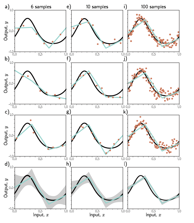
See the following figure from the book. It shows the effect of training with 6, 10, and 100 samples at each column. The best-fitting model varies a lot when we use 6 points, and the variation reduces with increasing the number of samples. When we use 100 samples, the model almost does not change at all.

Bias

The bias term comes from the inability of the model to describe the true underlying function. If we increase the complexity of our model, and as a result make it more flexible the bias reduces. This is usually done by increasing the number of parameters of the model.

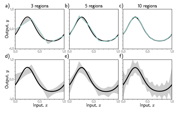
Check out the following figure again from the book. In this model, linear line line model is used in 3, 5, and 10 regions (dividing the interval of \([0,1]\) into 3, 5, 10 regions). As expected, increasing the number of regions, the model can better match with the original data. However as you see in the second row, the variance of the model is increased, since the model overfits to the data used. This is known as bias-variance trade-off.

Bias Variance Trade-off

The above figure showed a side effect of increasing the model complexity. Given a fixed-size training data, as we increase the complexity the variance term increases. So increasing the model complexity does not necessarily reduce the test error. This is what is known as bias variance trade-off.

The following figure shows this trade-off in another way. The first row shows that we fit three linear region to a sampled 15 points data (sampled three different times). All the time we find almost the same set of linear lines, meaning that variance is small. However, in the second row, we increase the number of regions to 15. Now the model better fits to the data points we sampled, however, each time we sample another dataset, we literally fit to the data, and we find a totally different fit. The model output varies given different datasets and shows the increase in the variance of the model given different sampled data. This is also known as overfitting. ![[Pasted image 20240221001728.png]]

Double descent

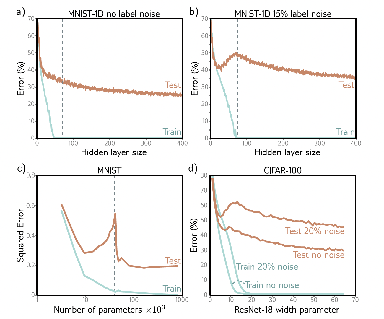
Consider this experiment: Consider the MNIST-1D dataset involving 10,000 training and 5,000 test examples. We then increase the model’s capacity and observed its impact on performance of the model. As the number of parameters in the model increases (model capacity increases), then the training error decreases to nearly zero (even before reaching a capacity equal to the number of training examples). Also we observe that the test error also decreases, which contradicts the expected increase in test error due to the bias-variance trade-off. Instead, test error continued to decrease, showcasing an unusual pattern (see following figure from the book)

A follow-up experiment with 15% randomized training labels reveals a similar trend in training error reduction. However, the test error initially followed the anticipated bias-variance pattern, increasing up to a point, but then unexpectedly decreased again with added capacity, even falling below earlier minimum levels. This “double descent” phenomenon, where error rates drop after initially increasing as capacity grows, was observed in both the original and noisy datasets, indicating distinct under-parameterized and over-parameterized regimes, with a critical regime in between where error rates peak. Similar patters also is seen on CIFAR-100 data with Resnet-18 network.

But why?

The concept of double descent challenges traditional understanding by showing that test performance first worsens as models gain just enough capacity to memorize data, then improves even after achieving perfect training performance. This contradicts expectations since over-parameterized models, with parameters outnumbering training data points, should not improve due to lack of constraints.

So when the number of parameters increases the model has enough capacity to fit the whole data with zero training loss. So it can fit the training data perfectly. So increasing the number of parameters would not result in the model fitting the training data better (since the loss is already zero)! So if anything happens is because of some-change that occurs for in-between training data, or how the model prioritize one solution over another as it extrapolates between data points (this is known as inductive bias). Inductive bias is the assumption that a learning algorithm uses to predict outputs given inputs that it has not encountered before.

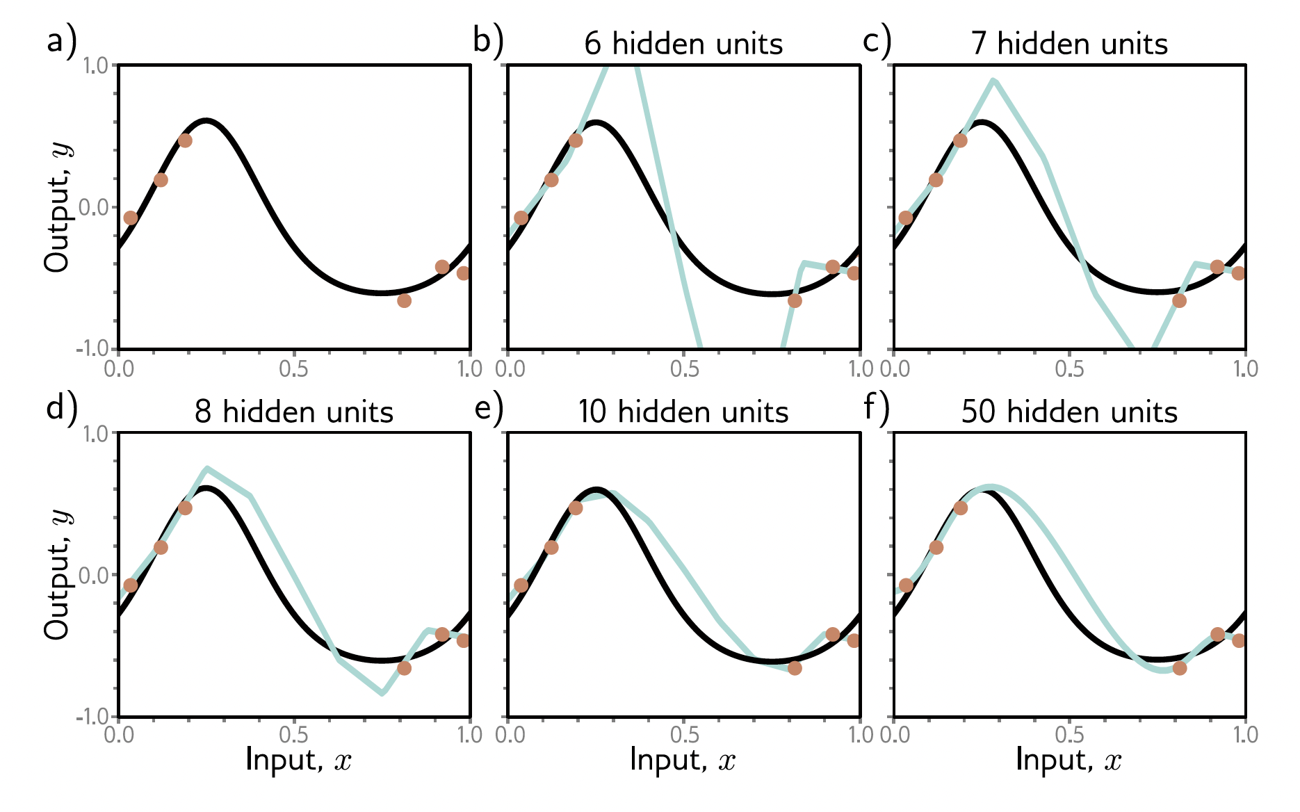
Note that the data is in high dimension. Considering the number of possibilities for input data and the number of data points we have, you can easily see that we have sparse data in high dimension, so the ability of the model to predict in-between training data points is very important. This situation is simplified to the following figure. we have a limited number of data points. Now you can see that as we increase the number of hidden-units in NN, the model predicts smoother functions between the datapoints. Commonly it is thought that in double descent as we increase the number of parameters in our model, it interpolates more smoothly between training data points, and hence generalize better to new data. Interestingly as seen in the following figure, when the number of hidden units are exactly the same as the number of datapoints, the output distorts to fit the data (similar to increase we saw in the test error for bias-variance trade-off cases above), but as we increase the number of parameters the function becomes smoother.

As capacity increases, models can create smoother interpolations between data points, which is believed to enhance generalization to new data. This phenomenon suggests that model capacity contributes to a form of regularization, guiding models towards smoother functions that better predict unseen data. However, the mechanisms driving this smoothness, whether through network initialization or the training algorithm’s inherent preferences, remain uncertain.

Essentially, the discovery of double descent reveals that adding parameters to a model beyond the point of memorization can lead to better performance, due to the model’s capacity for smoother function interpolation in the vast, sparse high-dimensional input space.